Question

Facebook Leads Ads i.c.m. Spreadsheet with pre-filled columns

  • 25 January 2023
  • 2 replies
  • 24 views

I want Facebook Lead Ads data to be connected to a spreadsheet (easy to set up), however, I want that data to connect with already prefilled in columns in that spreadsheet.

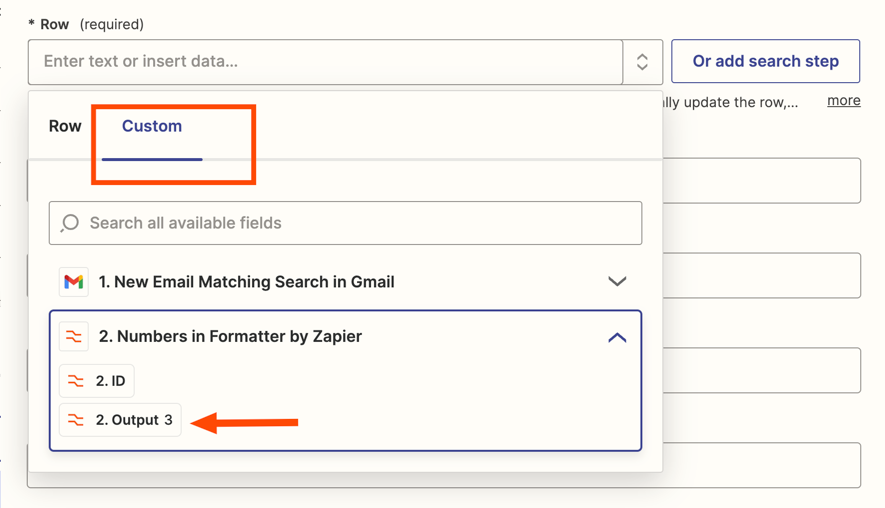
Columns A, B and C are being collected out of the Facebook Lead Ads data. But Column D is already in place with coupon codes. Normally, Zapier will put the Lead Ads data in the first empty row available (meaning: the first row were Column D is empty). However, I want Zapier to put the Lead Ads data in the first rows that are empty for Column A. This way, the Lead Ads data will be put in the same row as a discount coupon in Column D.

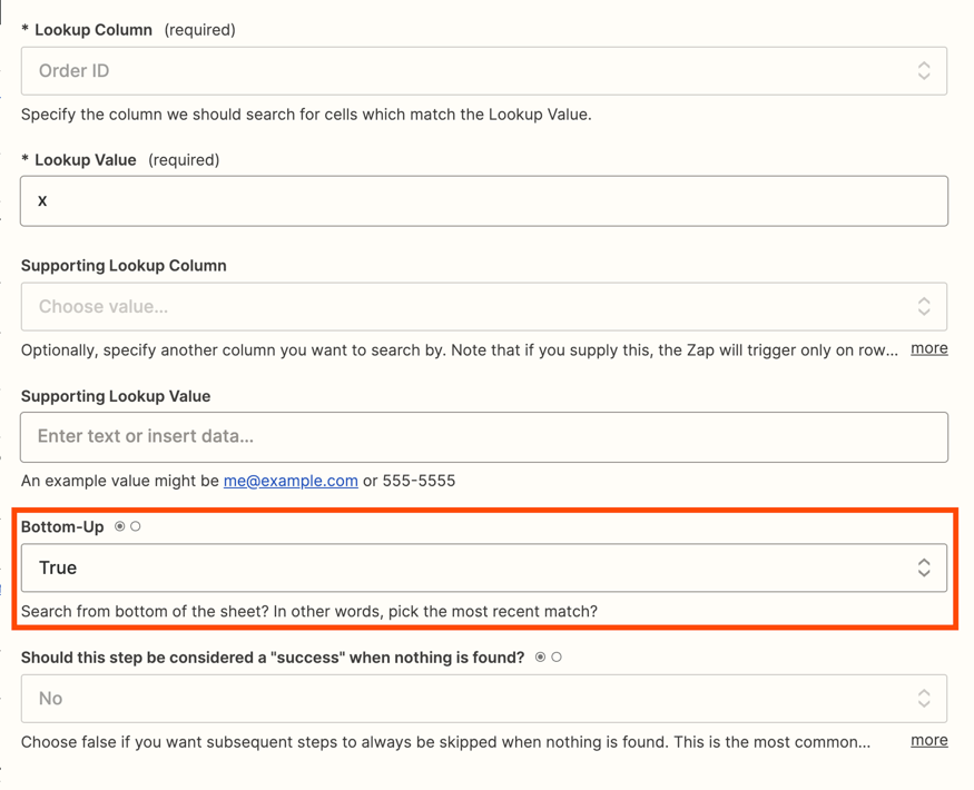
So, again: I know I should use the Lookup function in Zapier but I don't know how to set it up the right way. Anybody able to help me on this one?

I've made a video on Twitter about this: 


This post has been closed for comments. Please create a new post if you need help or have a question about this topic.

2 replies

Userlevel 7
Badge +14

Hi @Maatwerk Online 

Good question.

Add another column (e.g. USED) with a value (e.g. NO).

Then use the GSheets Lookup Row to search (top down) for the first row with a value of NO in the USED column.

Then use the GSheets Update Row step to update the found row by populating the desired columns from Step 1 and changing USED = YES.

Userlevel 7
Badge +12

Hi @Maatwerk Online!

You’re very close to getting it - you do need to use the Lookup Spreadsheet Row action. 

You’ll need to set up a lookup step that searches for a value in a column that will be the same in every row with Facebook data. If there’s nothing currently in the sheet like that, add a column to the sheet and put an x in every row with a lead already in it

In the lookup step, set the Bottom Up value to true


The search will start at the bottom of the sheet and go up until it finds the first row with an X in it. We now have the Row ID for the most recent row that has Facebook Lead Ads information in it. 

Next we need to add 1 to that value so that the update Spreadsheet Row step updates the first empty row. The easiest way to do that is with a Formatter step, you can use Perform Math Operation or Spreadsheet-style formula, whichever you prefer. To sum up this step: you’re taking the row ID found in the Lookup step and adding 1 to it. 


Then take the output of the Formatter step and use that as a Custom Value for the Row field in the Update row step. 

That action will then update the first row that doesn’t have data in it (other than the coupon). If you’ve added a column to search (one filled with x’s), make sure that you also update that column in the update row step so that the next time the Zap runs, it’ll find the correct row. 


To sum up, here’s the steps I’d use:

  1. Lookup Spreadsheet Row
  2. Formatter > Numbers (add one to the row ID found in the previous step)
  3. Update Spreadsheet Row (use the output of the Formatter step to select the row)


I hope that’s all clear, let me know if you have any questions :)


That’s how I’d do it, if anyone has any thoughts on other ways to achieve the same thing (maybe with less steps?) then let us know!