

Mod Edit: 03-17-2022
Have you ever wanted to create a row in Google Sheets, and use a formula that references another cell in that row? If you’re in Google Sheets, you could just copy and paste that row, and the cell references will change automatically. But normally in Zapier, you have to do this:
-
Create the new row so that we get the Row number
-
Update the row with the formula using that Row number
That’s because when we create a new row, we don’t know what the row number is going to be until after we create it! So we have to add the formula after we know the row number, which uses up two tasks to create just one row.
But with a little bit of formula magic we can save that second task every time. We can do this by using INDIRECT and ROW.
INDIRECT lets us use formulas to reference other cells. Normally if you wrote a formula like "SUM(A3,"B" & 3+3), this would not work because formulas will not work as cell references. In other words, this would not resolve to "SUM(A3,B6)", and we would just get an error. However, if you surround that last bit with "INDIRECT," it will work.
In other words:
=SUM(A3,INDIRECT("B" & 3+3))
Will resolve to:
=SUM(A3,B6)
That might not seem very useful on its own! But in Zapier, we can combine this with ROW() to reference a cell in the row we’ve just created, and skip having to update it with another action!
Let’s say your Zap is putting two numbers in columns B and C, and you want the total of those numbers to show up in column D. In Google Sheets, you would simply write:
=SUM(B2,C2)
into D2, and copy that from Row 2 into all the other rows. In Zapier, you can do something very similar, but it would look like this instead:
=SUM(INDIRECT("B" & ROW()),INDIRECT("C" & ROW()))
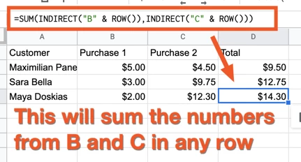
That looks complicated, but it’s actually pretty simple when you break it down step by step! When the Zap runs, ROW() will equal the row that it is in. If the Zap created row 88, then the ROW() formula would resolve to:
=SUM(INDIRECT("B" & 88),INDIRECT("C" & 88))
Then the INDIRECT formulas would take those strings, and turn them into cell references like so:
=SUM(B88,C88)
And voila! A formula without any extra tasks. You can use this to perform calculations on other cells, run IF statements based on other data, and more! All without using another task.
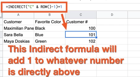
BONUS: Use INDIRECT to reference cells in completely different rows
The great thing about INDIRECT is that you can use it to reference any cell, based on whatever math you like. Let’s say you wanted to check if the previous row had an odd number in column C. You could use this formula:
=ISODD(INDIRECT("C" & ROW() - 1))
See what’s happening there? We’re subtracting 1 from the ROW number of the cell we just filled in. So if this was in Row 88, the formula would resolve to:
=ISODD(C87)
And in that way, you can reference a cell anywhere in relation to the row you just created! I’ve seen people use this to set up warnings when a number got too high, assign unique IDs based on previous rows, and more. Here’s an example of creating a new Customer number based on the previous row:
Alternatives:
With Google Sheets, there are usually about 50 ways to do the same thing! Here is a great post on how to use the original, two-step version to create dynamic formulas.
UPDATE:
For those of you using large Google Sheets it may be better to use use INDEX instead of the INDIRECT function as per GetUWired’s suggestion below. This should help to prevent any potential performance issues:
The formula
=SUM(INDIRECT("B" & ROW()),INDIRECT("C" & ROW()))would be come
=SUM(INDEX(B:B, ROW(),1),INDEX(C:C, ROW(),1))


") I may just take you up on that offer to get some extra context/examples!
I may just take you up on that offer to get some extra context/examples!