I have a zap that looks up a spreadsheet row in Google Sheets when someone books a new appointment in Acuity. If it doesn’t find an existing matching row, it creates a new row. 

I also have a second zap that strikes through a row when someone cancels an appointment in Acuity. 

The problem is that, if the last row on the sheet is formatted with a strikethrough, any new rows that are added are also formatted that way. I tried conditional formatting any empty cell in the spreadsheet to not have any formatting as suggested in a similar post, but that hasn’t worked either. 

Any ideas for workarounds?

Thanks!

Hi @SSDT 

Since Zaps adds a new row when it creates a row (vs populating the next open row) that is why the new row inherits the previous row’s styling.

You’d have to do a similar execution to clear the row formatting as you did to set the strike thru formatting.


Hi Troy,

I tried doing this via a filter after the step that adds the strikethrough formatting but I’m still having trouble.

My process:

  1. Acuity Scheduling Appointment Canceled​​​​​​​
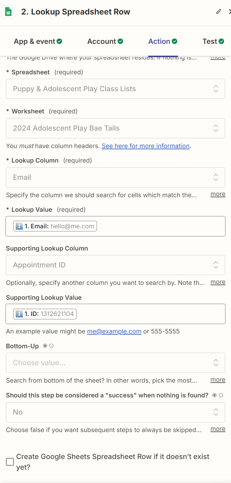
  2. Lookup spreadsheet row (by email & appointment ID)
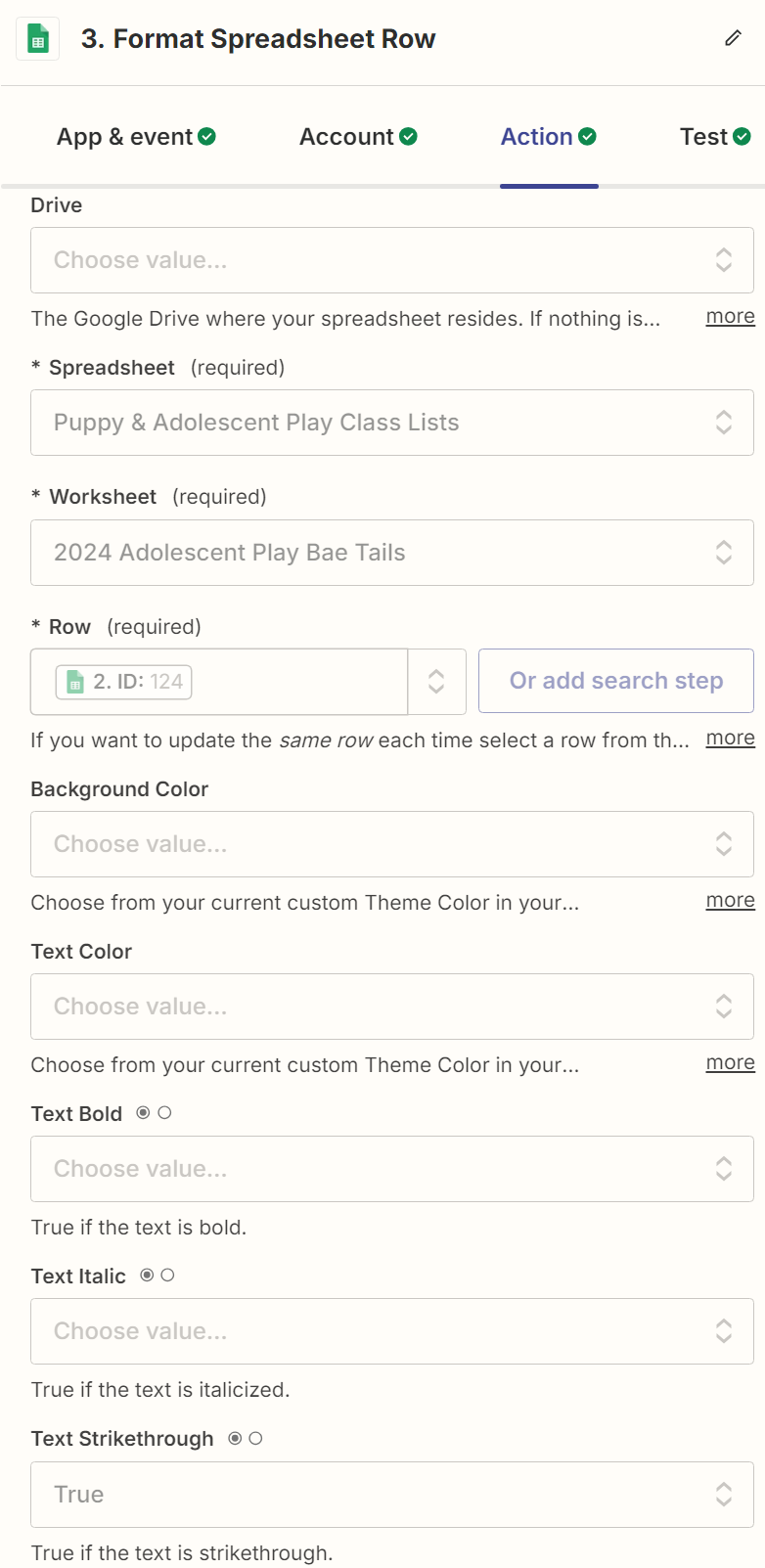
  3. Format spreadsheet row (text strikethrough: true)
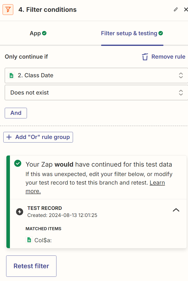
  4. Filter by Zapier (only continue if Column A data does not exist - so a blank row)
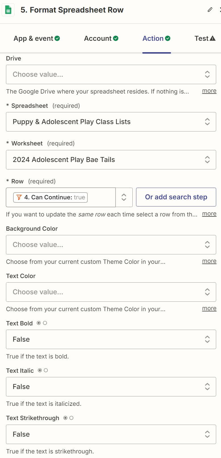
  5. Format spreadsheet row (with the row as 4. Can continue: true, and text strikethrough: false)

Though the step 1-4 tests work, step 5 always returns this error: 

Any additional advice? Thanks for your help!


@SSDT 

For us to have more info, post screenshots with how your Zap steps are outlined and configured in EDIT mode.


  1. Acuity Scheduling Appt Canceled
  2. Lookup Google Spreadsheet Row
     
    1. Format Google Spreadsheet Row


    2. Filter for blank spreadsheet row 


    3. Format Google Spreadsheet Row

My hope is that this will create a blank row at the bottom that has no formatting, so when a new row is created (with a different zap), it will not automatically have strikethrough formatting.

Thanks again!


@SSDT 


Step 5 is not configured correctly for the Row field.


Step 3 for reference.


Step 3 is done with a lookup of a specific row (by email & appt ID), and I need Step 5 to apply to the first blank row. Can I achieve that with a lookup step instead of a filter?


@SSDT 

The Row field expects a number value. (“true” or “false” are not valid values from Step 4)

If you are trying to format the first blank row (not the row from Step 3), then you may need to add another GSheet Lookup Step (or possibly use the GSheet API).


Hi @SSDT 👋

I wonder if you could get around this by having two worksheets set up in Google Sheets for this, one connected to the Zap that adds the new rows of information. And another that’s connected to the Zap that adds strikethrough formatting to specific rows. The second (“strikethrough formatting”) worksheet could use the Google Sheets IMPORTRANGE formula to pull information from the first worksheet. I’ve not tested this myself but I’m thinking that approach would get the new rows added to the second spreadsheet without the strikethrough formatting being copied to the new rows. 

Do you think that could work? If you do give that approach a try please do let us know whether or not it works. Would love to know if it definitely works as hoped! 🤞


Reply