Best answer

Search for Column - Google Sheets

  • 26 June 2020
  • 2 replies
  • 439 views

Userlevel 7
Badge

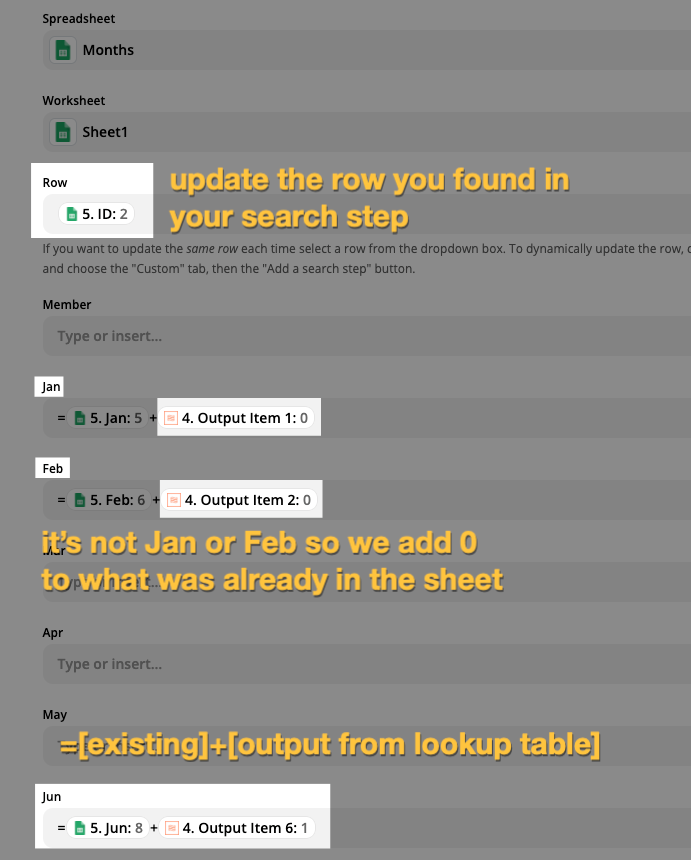
I have a zap that updates numbers of leads per member onto a spreadsheet by finding Row ID then using formatter to add 1 to existing total every time a new lead comes in. 

However I now want to split the updates according to month of year. So that I can quickly see x number of leads for member y in Jan, x number of leads for member z in Feb etc. rather than just the total leads per member for all time (as I have at the moment). 

To start with I would create 12 new columns in my spreadsheet for each month of the year. This would replace the single “leads” column I presently have (which is the column the +1 is added to each time)

If G Sheets had a “search for column” integration then I could use the date stamp of the Trigger, convert it to month via formatter step and then search header row for matching Column month. Then I could use that column as the the column to update in the original zap. 

But alas, there is no such integration for G Sheets (or Airtable). Nor is there one in Integromat.

I’m trying to get my head around another way to acheive this. Maybe there is a way with another app that I am totally overlooking? Google Calendar perhaps? Or maybe somebody has a javascript or Python code step that I could use to achieve my goal?   


icon

Best answer by nicksimard 27 June 2020, 01:18

View original

This post has been closed for comments. Please create a new post if you need help or have a question about this topic.

2 replies

Userlevel 7
Badge +11

Hey @ChrisP!

Just to make sure ai understand what you mean, are you saying that you’d have 12 columns in the spreadsheet and depending on which month your Zap triggered in, you would update the corresponding column by adding 1 to the number that’s already there?

So if it triggered today you would want to take the value in your June month and increase it by 1. Am I understanding that correctly?

I came up with a workaround, but it does eat up some tasks in order to do it. A single Code step would be ideal (maybe someone else can offer that), but I’m not familiar enough with that to craft something. But workarounds, I got plenty of those 🙂 
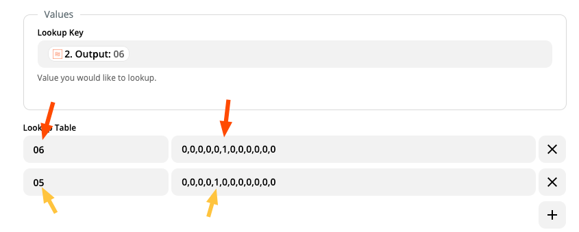
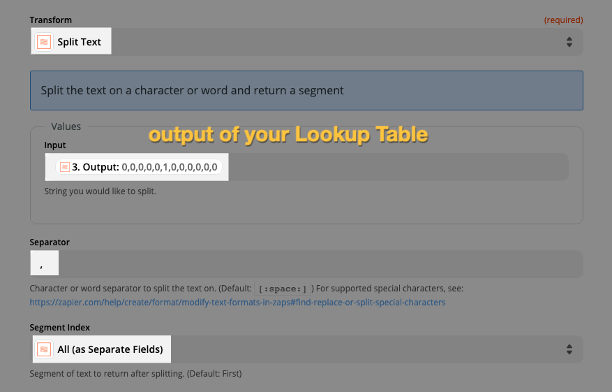
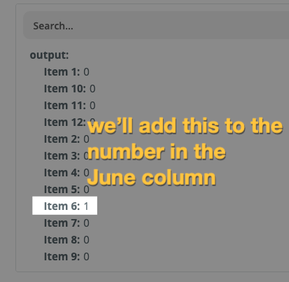
Here’s what I came up with (this would be after your Formatter step to get the month as a number):

Formatter — Utilities — Lookup Table

Depending which month comes through, you’ll output a series of 0s and just a single 1 in the place for that month. So 6th month, the 1 is in the 6th position. For the 5th month, it’s in the 5th position.


Formatter — Text — Split Text

Next, you’d take the output of that Lookup Table and split that text, by the comma, outputting each of the parts as their own separate fields.

That gives you something like this:


Google Sheets — Lookup Spreadsheet Row

Find the row for the member that you want to update. This part is pretty straightforward. Next, we’ll put all the pieces together.

Google Sheets — Update Spreadsheet Row

You’ll update the row that you found in your search step, and map each of the separate fields like this:

You have to add the formula right into the Zap like this:

=[the-existing-value-from-Google-Sheets]+[the-corresponding-output-from-lookup-table]

So output item 1 goes into the January column’s formula, output item 2 into February, and so on.

Wrapping Up

Again, I’m essentially working around the fact that I’m not able to create the code that would do that same thing. That forces me to come up with workarounds using other apps in Zapier. Hope this helps!

Userlevel 7
Badge

@nicksimard Genuis! Excellent work around which will solve my problem. Thanks! :thumbsup:

If anybody out there does have a code step it would be great, but in the meantime I am definitely going to implement this.