@leadrouter
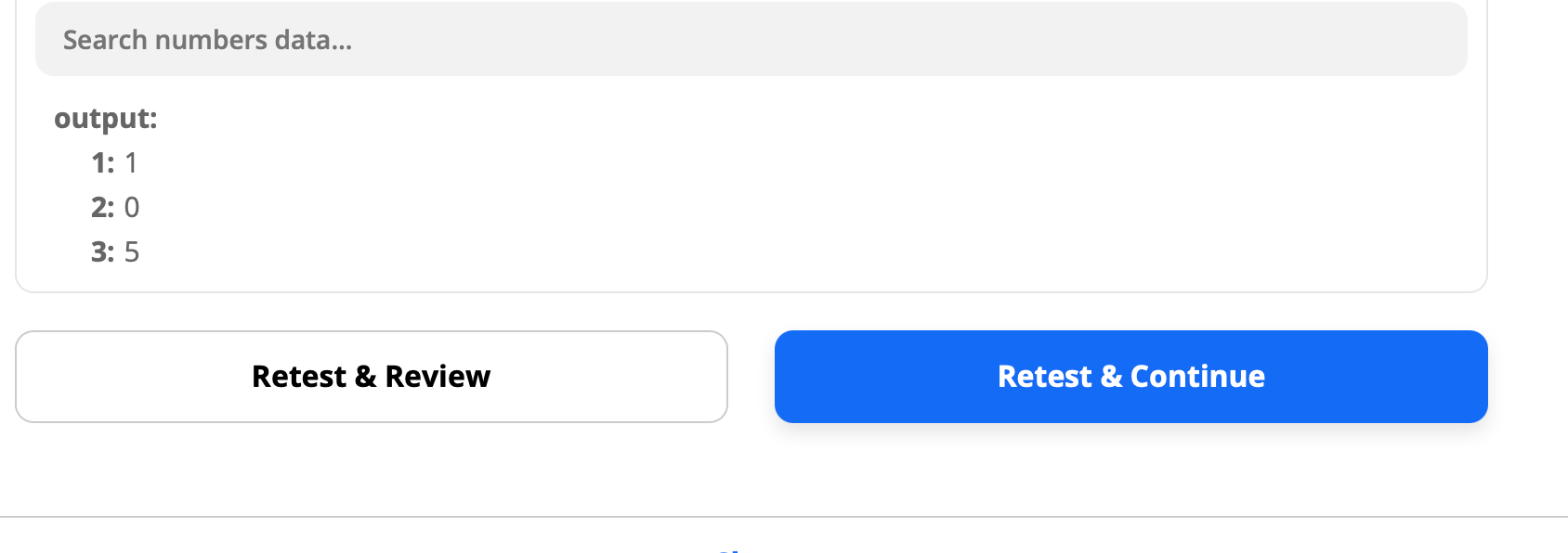
> I am wondering if it does not consider the field to be a number
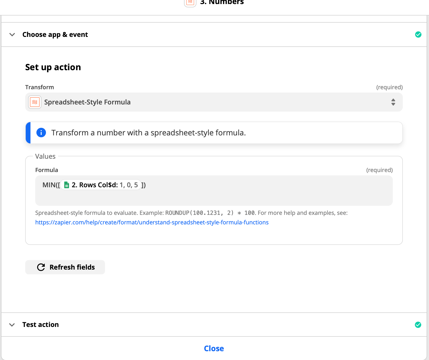
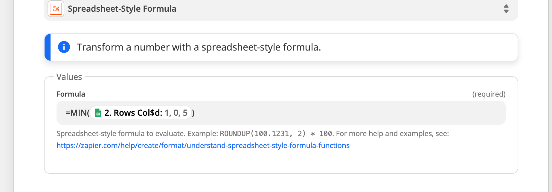
I think you’re right! Based off that screenshot it looks like we’re trying to format an array of numbers, but this is not easy to see in the Zap editor.
Can you try this:
-
Add a Formatter > Utilities > Line-item to Text action, and map the output of your Google Sheets step there (the “1,0,5”)
-
This will turn that into a string of 1,0,5
-
Send that string ^ to the formatter step you have with the spreadsheet style formula. Based off that, it should return “1”
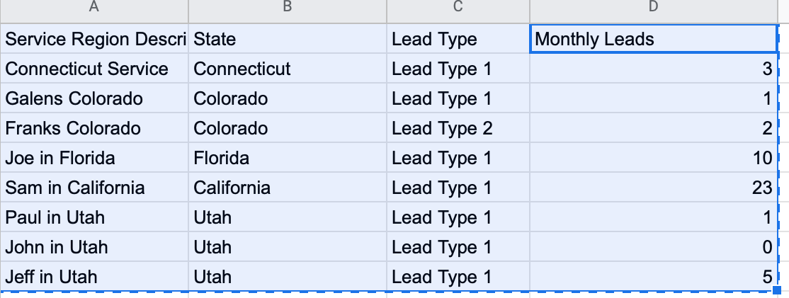
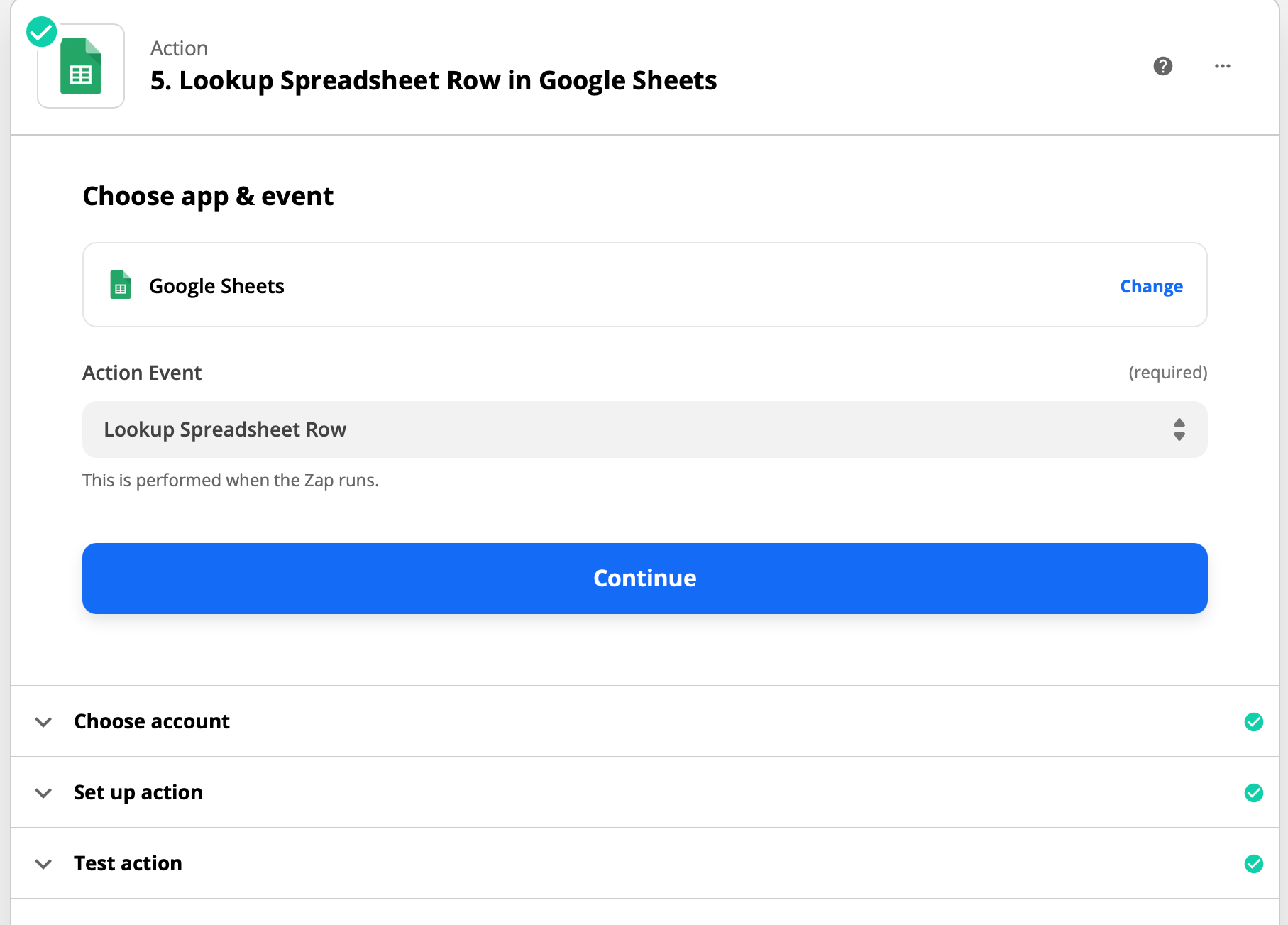
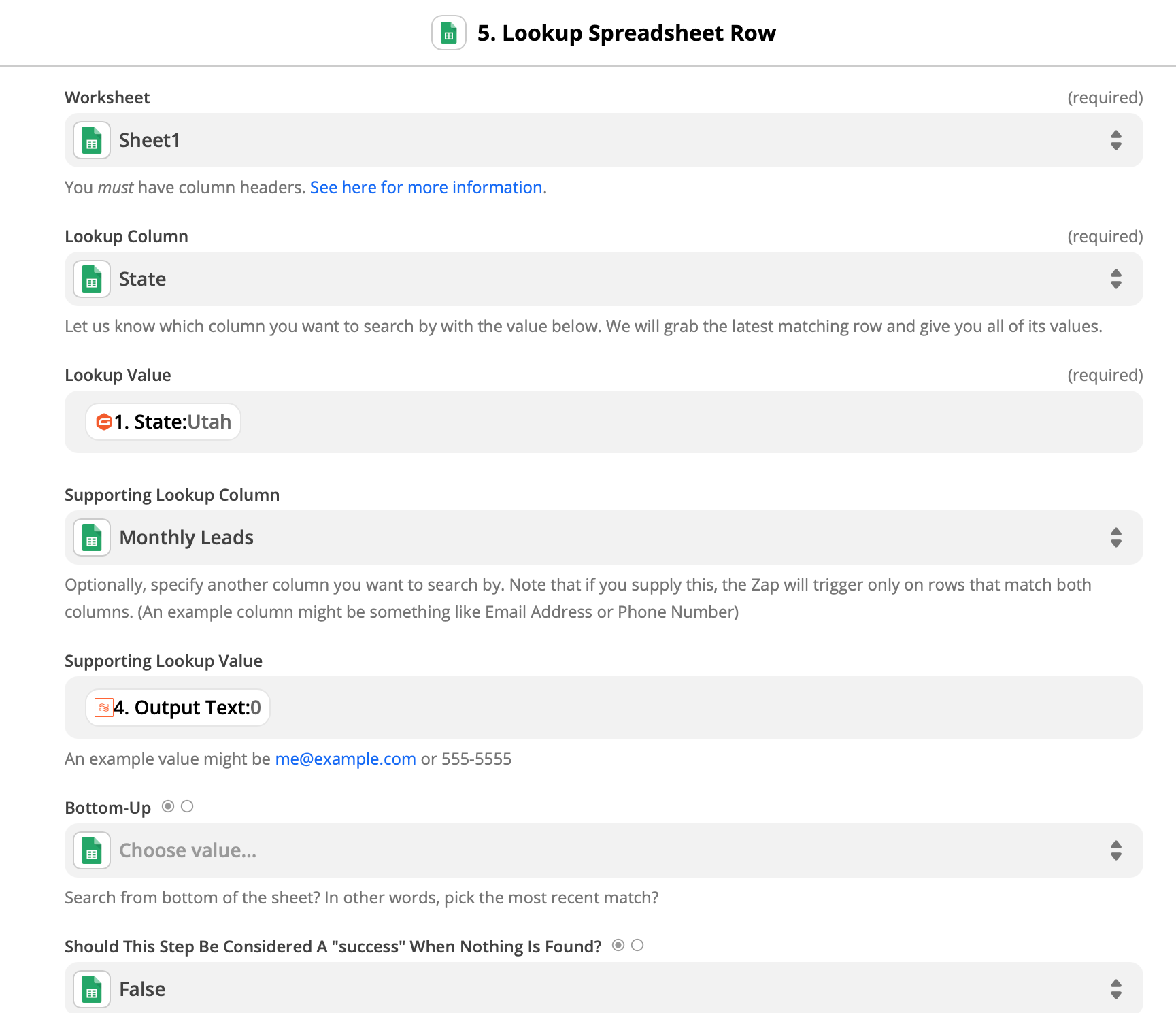
After that it sounds like want to reference the row that matches “Utah” and “1” - which I think should be doable with another Lookup Spreadsheet row action, using a two column search.
Let me know if this helps!

")