Best answer

Creating an Automatic Hour Tracker Via Google Spreadsheets and OpenPhone


Userlevel 2

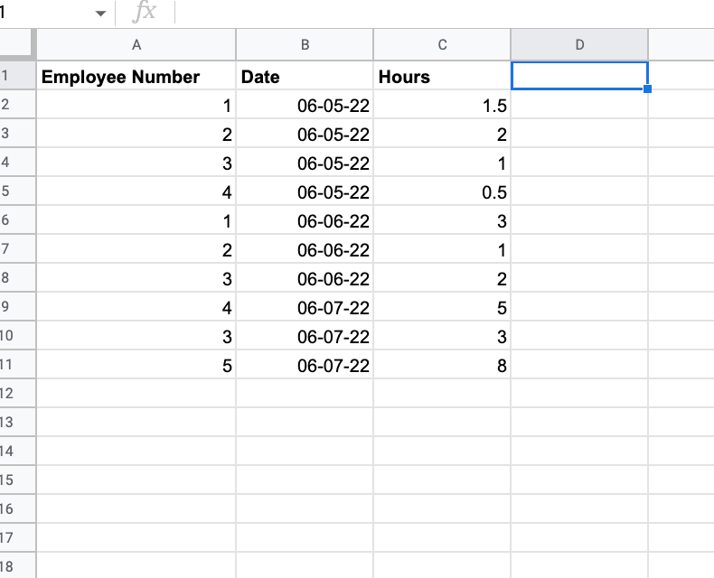
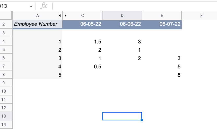
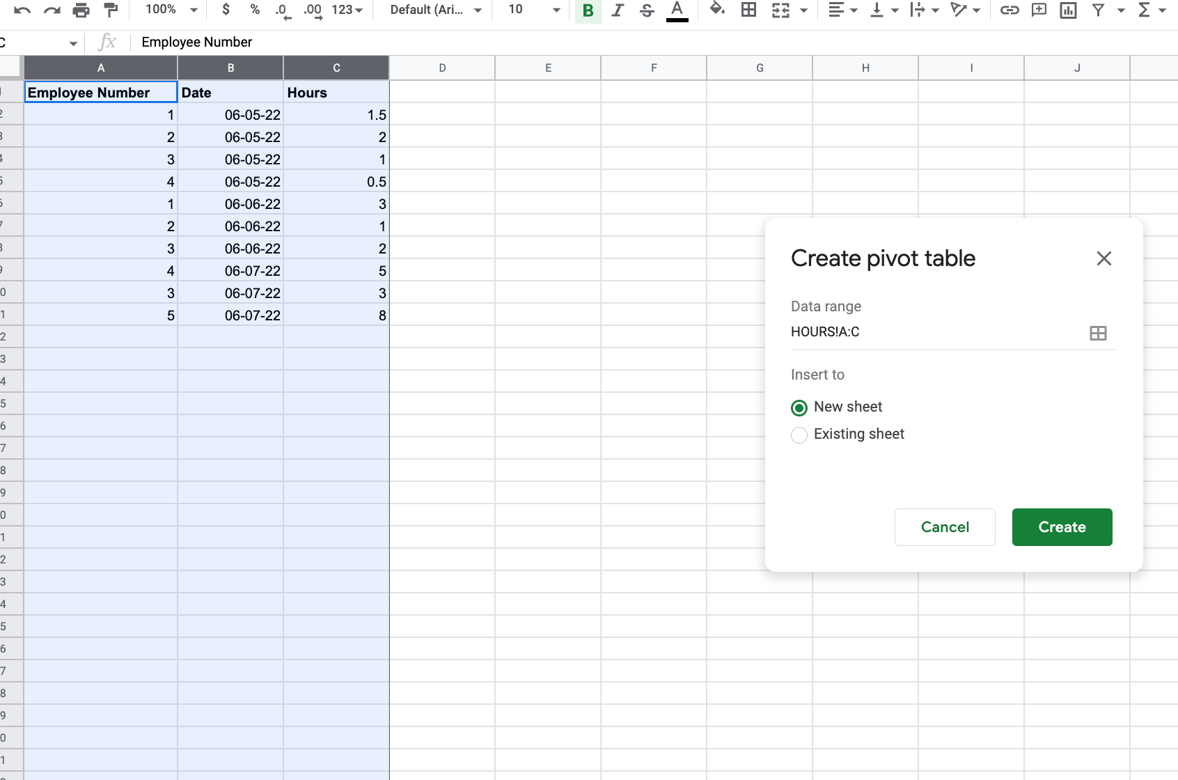
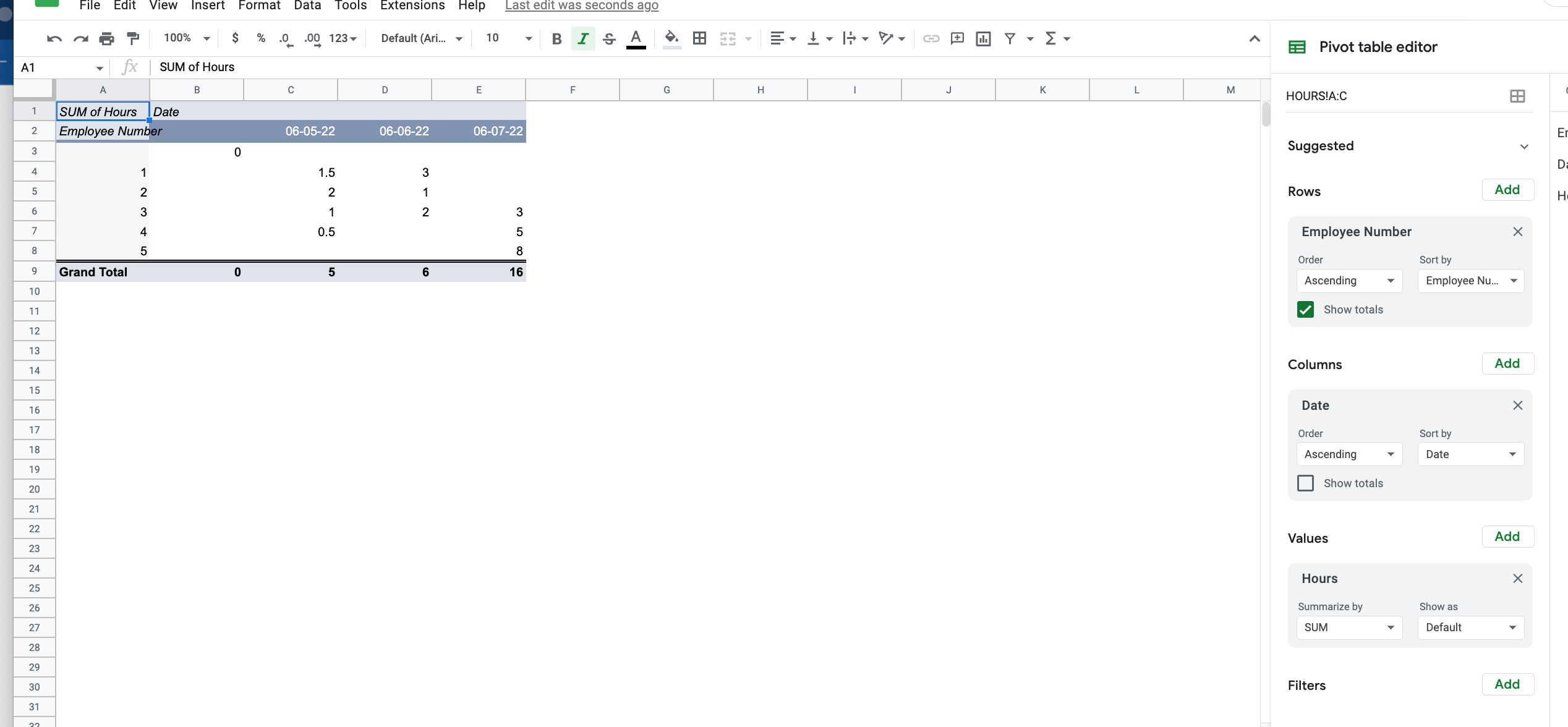
Hello Everyone! The idea is to have an employee send the number of hours they worked that day to a phone number power by OpenPhone. The Zapier integration recognizes that the employee has a number and looks up spreadsheet rows for the number. If the number isn’t in the spreadsheet then it is added in as a row. So far so easy. The hard part is placing the entered hour into the right column and row according to the day the message is sent. I tried using OpenPhones creation date, formatting it into a normal date, and looking up that date in Google Sheets but I constantly get the error “There was an error writing to your Google sheet. Unable to parse range” for the date of the column. I also don’t have a lookup value. I’m not entirely sure how to place the employee’s amount of hours in the correct column for the date they sent the message and the correct row beside their name. I’ve included a few pictures to illustrate what I’m trying to create. I know I suck at explaining things. I have an automatic zap that creates a new column with that days date at midnight. 


Please help big brain geniuses of zapier. It’s super hard to have the hours only go to the date the message was submitted even though the data for that is there. Having is place it in the correct row is difficult too.


Excuse spelling, typed at 12 am. 

icon

Best answer by GetUWired 6 June 2022, 17:08

View original

This post has been closed for comments. Please create a new post if you need help or have a question about this topic.

5 replies

Userlevel 7
Badge +12

Hi @jkrocks47 

This would not be possible with the current way Zapier handles columns in Google Sheets and with your current set up. As you are adding Columns in your first zap, your second zap would have more an more input fields (one for each column header on your sheet). It would not be easily possible to dynamically set these as the integration grows.. the input fields would need to be set from the beginning.

Instead… consider having a zap that just pushes your data to a totals sheet with 3 columns, Employee Number, Date, Hours

And then using a pivot table to translate the data into your desired output. Screenshots shown below with sample values. 

Master sheet. 


PIVOT TABLE


To set up a pivot table. Highlight all the columns you want to display then (COL A, B, C in example) then click insert pivot table. Insert it into a new sheet. 


Then on your pivot table sheet you should see some config options. Configure as shown. You can then choose to hide row 1 and col B for the final output shown in the above example.


Userlevel 2

Following up

Userlevel 7
Badge +9

Hiya @jkrocks47! Were you able to review @GetUWired’s reply? They provided some amazing tips I think maybe useful. Keep us posted! 🤗

Userlevel 2

Hiya @jkrocks47! Were you able to review @GetUWired’s reply? They provided some amazing tips I think maybe useful. Keep us posted! 🤗

Thank you for the @. I didn’t see it at first. Perfect solution! 

Userlevel 2

@GetUWired YOU’RE A GENIUS 

 I had a similar idea to this, but I’m a noob with the google sheets/excel so I had no idea how to link them. I truly appreciate your help.