


I 🧡 Google Sheets.
My Zap workflows are full of Sheets triggers and actions - and if I have a tricky problem to solve - I often look to Sheets first for a solution.
One common use of any Spreadsheet App is formulas.
And when creating Sheets rows from a Zap - we’ll often want to apply existing formulas to the new rows we create.
There are already 2 fantastic Zapier Community posts on how to do this using 2 Steps in your Zap or the INDIRECT and ROW functions in Sheets.
Today I’m going to cover a 3rd option using Google Sheets Array Formulas.
The Issue - New Row Created After Rows with Existing Formulas
In a previous post - I covered how we can add extra data to a new Facebook Lead Ad by saving data to a Google Sheet and using the Sheet to do a VLookup.
I want to expand that Zap to keep track of my leads on the Google Sheet - and I want the new rows to look up the same data.
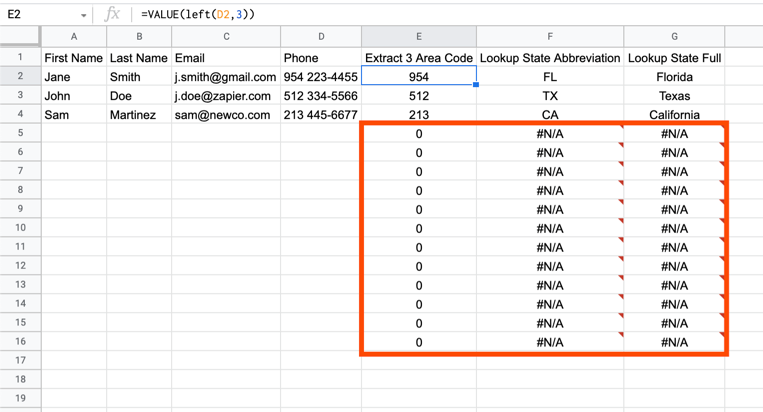
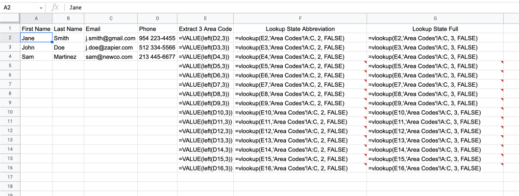
Normally - when we add Formulas to a Google Sheet - we copy them down the page.
The Sheet will look similar to this below - where we see 0’s or #N/A for formulas that don’t yet have data to calculate.
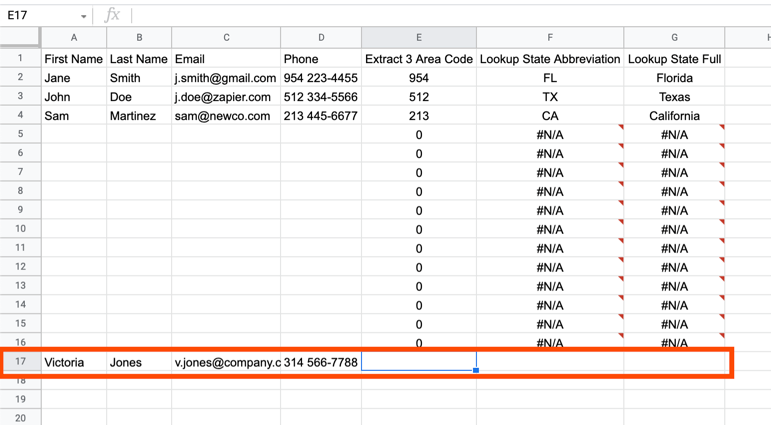
From a Zap - when we try to Create a Spreadsheet Row on a Sheet structured that way - something unexpected happens.
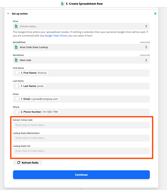
The Row is added to the next blank row and our formulas do not get applied.
This is where Array Formulas can help us.
Array Formulas - One Formula for the Entire Column
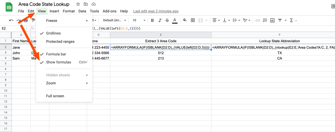
I’ve temporarily changed my Sheet to Show the Formulas - and we can see that with the typical setup - a Formula exists in every Cell from E2 to G16.
Array Formulas work differently.
With Array Formulas - we only put the formula in Row 2 (the first row after the Headers) - and Sheets will automatically apply that formula all the way down the Column.
While I’ve made the changes below in Columns E, F and G - let’s just focus on my original formula in Column E above.
The original formula in Cell E2 was:
=VALUE(left(D2,3))And then as we copied that formula down the page - the Column D reference would change to match the row - so in Row 4 for example - the formula was:
=VALUE(left(D4,3))
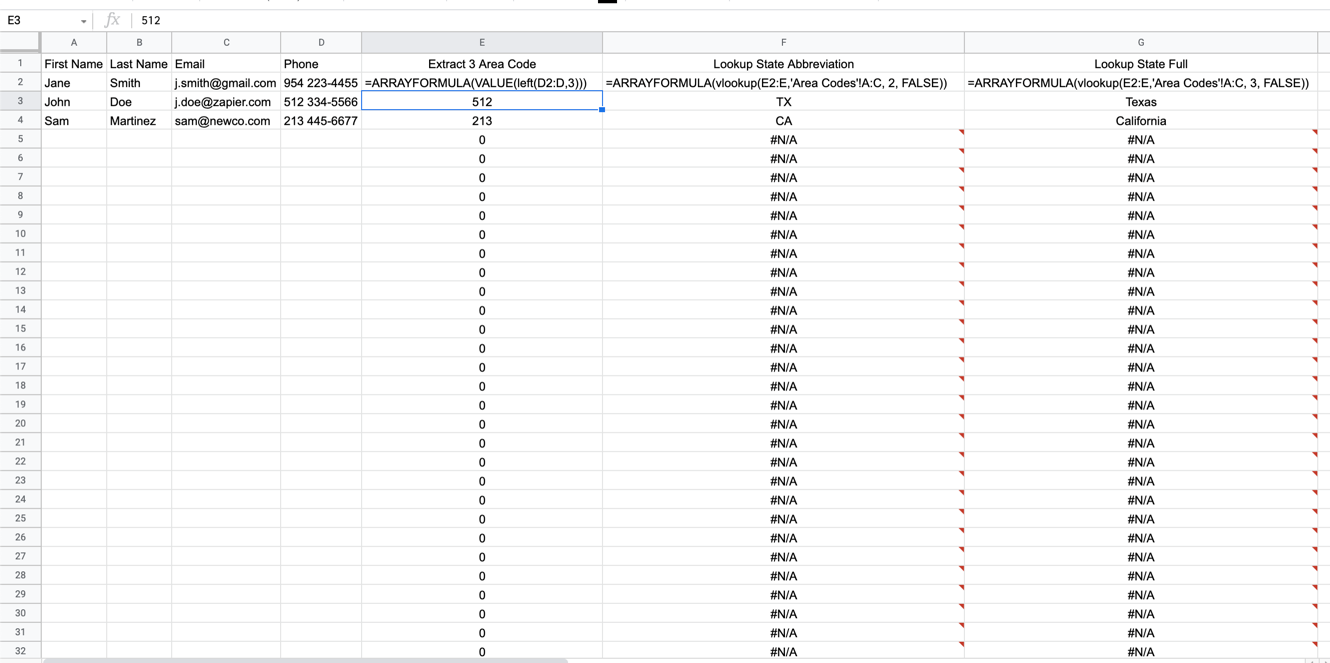
In my screenshot below - I’ve made 2 changes to the formula in Column E.
First - I’ve wrapped my original formula in ARRAYFORMULA() - this will apply the VALUE() formula to the entire column.
Second - I’ve changed D2 to be D2:D - this will tell Sheets to find the matching value for Column D by Row.
My formula now is:
=ARRAYFORMULA(VALUE(left(D2:D,3)))And then finally - note that I’ve deleted all the formulas from Row 3 down - the Formulas only exist in Row 2.
And notice what happens.
Even though the formulas only exist in Row 2 - the formula values in Row 3 and 4 calculate correctly!
This is the power of Array Formulas!
Testing Create Row with an Array Formula
So far so good - now let’s test our Create Row action again and see what happens.
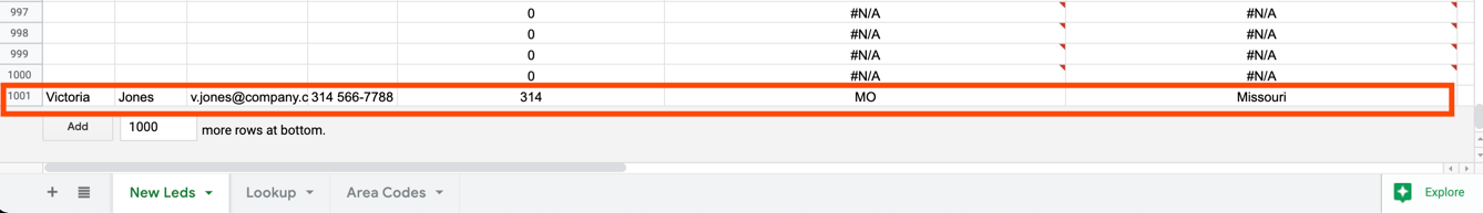
Uh oh.
Well the good news is our Array Formulas worked - the bad news is the row was still created in the next blank row that didn’t have any array formula values in it (row 1001).
IF() and ISBLANK() to the Rescue!
Luckily - we’ve got a fairly easy fix here.
We’re going to make 2 more adjustments to our formulas in Row 2.
Again - I’m going to focus on just column E.
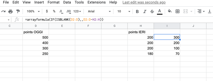
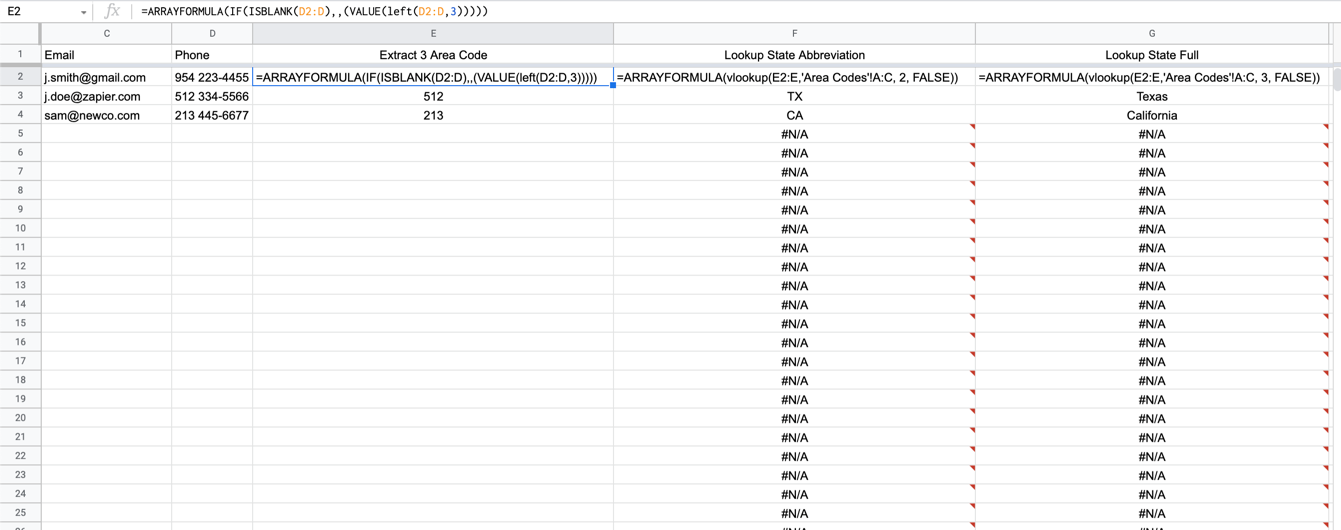
Right now - our Array formula is applying to every row on the Sheet - but we only want it to calculate when there is actually data in the Phone Column - Column D.
So we’re going to adjust our array formulas so IF column D ISBLANK - the formula doesn’t run.
To do this we’ll add this below just after the ARRAYFORMULA part of our formula in Cell E2:
(IF(ISBLANK(D2:D),,And then we’ll also add the closing parenthesis at the end of the formula.
Now our entire formula is:
=ARRAYFORMULA(IF(ISBLANK(D2:D),,(VALUE(left(D2:D,3)))))If we’re “reading” that formula from left to right - we’re basically telling Google this:
- Apply this formula to the entire column
- If there is no value in Cell D for the row - then do nothing
- If there is a value in Cell D for the row - then apply the VALUE() formula to that row
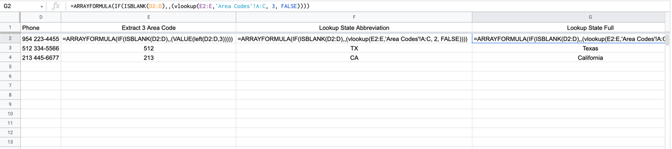
In the screenshot below - I’ve only made the change in Column E to illustrate the difference after adding the IF() and ISBLANK() functions to our formula.
Notice that our Array Formula in Column E now stops at row 4 - but in Columns F and G (where we haven’t applied IF and ISBLANK) - the formulas still run all the way down the Sheet.
Putting it All Together and the Final Test
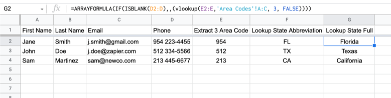
OK - now let’s make the same IF and ISBLANK changes to our Array Formulas in columns F and G.
And as expected - now we see there are no populated rows past row 4 which is the last row with data in column D.
So I’m going to switch my Sheet back to Hide the Formulas.
And now even though we can only see them in the Formula Bar - the Array Formulas are there in Row 2 - ready to do their work.
Finally - let’s run one last test to create a new row from our Zap.
And...Success!
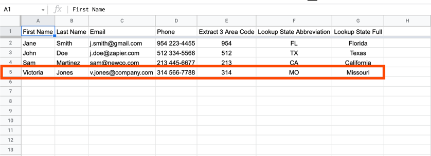
Our new row is created in Row 5 - the next blank row on the Sheet.
And our Array Formulas in Columns E, F and G are applied to the new row as expected.
Summary
When creating new rows on a Google Sheet from a Zap - the new row will be created in the next blank row on the Sheet.
This means existing formulas which are applied to the entire column won’t apply to the new row that is created.
There are multiple solutions for this (2 others are linked in the introduction above).
The Google Sheets Array Formula is a powerful 3rd option.
The Sheets ARRAYFORMULA() function enables us to enter the formula in Row 2 of the Sheet - and have that formula apply to any New Rows added to the Sheet.
By combining the Array Formula with IF() and ISBLANK() functions - we’re able to Create New Rows on the Sheet and apply all existing formulas.
And we’re able to do this without leaving any blank rows in between the existing row and the new row we’ve created.
I hope this post enables you to build more useful Google Sheets Zap workflows!
If you do give Array Formulas a try - I’d love to hear about it in the comments below. :)