


Hi, I’m Clint, a Customer Champion at Zapier! I’m obsessed with Google Sheets, Zap loops, and edge cases. This Wednesday, I’d like to discuss using multiple IF statements to score a lead based on specific criteria.
The Challenge
I had a customer recently whose goal was to score leads based on special criteria they had determined to be important. For example, if a customer said they had an immediate need, they would get 1 point. If they were also in the Manufacturing industry, they would get an additional point. In this way, you could tally a final score for that Lead.
The Solution
Initially, we were working on using a series of Paths and math formulas, but that wasn’t working very well. Instead, I finally realized I could use my favorite formatter, the Spreadsheet-Style Formula, and a few IFs added together.
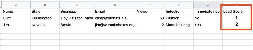
Let’s look at the leads first so we can get an idea of what kind of data we have to work with:

The three highlighted columns will be used to score the lead. They’ll get 1 point if they’ve viewed our page >20 times, 1 if their industry is Manufacturing, and 1 if they have an immediate need, for up to 3 possible points.
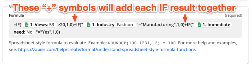
Now we know what we’re working with, so it’s time to build a formula. We’ll use an IF statement to generate either a 1 or a 0 for each of those, then add them all up. The first IF formula would look something like this:
IF({{Views}}>20,1,0)What this is saying is “If the Views number is greater than 20, return the number 1; otherwise, return the number 0”. In the first row, this would return 1. The other statements would be:
IF("{{Industry}}"="Manufacturing",1,0)and
IF("{{Immediate_Need}}"="Yes",1,0)Notice the quotes around these fields - any time we’re using text, we have to make sure to use quotes, or the formatter will get confused.
The last thing to do is to add them all up. This is easy enough - just put a “+” between each IF formula. At the end of the day, we get something like this:
If we were to run that exact formula, we would get a result of “1”. Now all we need to do is pass that back to Google Sheets in an Update Row action. If we run this on both rows, we get the following result:
So rather than using up to 6 formatters for this, we can get it all done in one! And this one step can handle as many criteria as needed - you can just keep adding IF formulas to the end.
Wrapping Up
I think this shows how flexible the Spreadsheet-Style formula is - it runs as many valid formulas as you put into it, meaning you can do a lot of interesting things.
What kinds of formulas have you used? Let me know, I’m always interested in hearing about your cool formulas!