Hey there, Zappers! Following up on our intro article about spreadsheet-style formulas, let’s dig into some more detailed examples of how to use them in your Zaps. We’re going to start with something that a lot of people use in their Zaps: IF/AND/OR statements.
What We’ll be Covering
IF Statements
IF(Something is True, then do something, otherwise do something else).
IF/AND Statements
IF(AND(Something is True, Something else is True), Value if True, Value if False)
IF/OR Statements
IF(OR(Something is True, Something else is True), Value if True, Value if False)
Nested versions of the above.
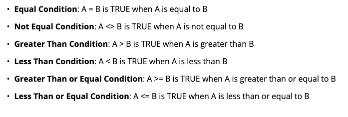
NOTE: The “something” above can be any of the following:
Let’s Start With Something Pretty Basic
Before we get to complex examples, let’s ease into things first with a few easier ones.
IF | Two Strings Match, Output Value 1, Otherwise Output Value 2
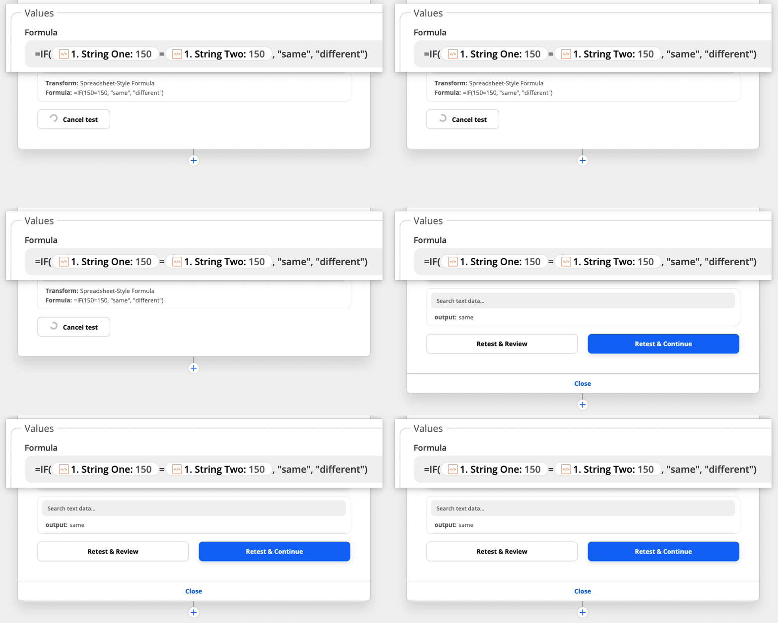
Let’s say you want to compare two strings (these could be words or numbers) to see if they match. If they do, you want to output value #1. If they don’t match then you want to output value #2.
=IF(“string1”=”string2”, “same”, “different”)
In a Zap:
IF / AND | String A Matches String 2 AND String 3 Matches String 4, Output Value 1, Otherwise Output Value 2
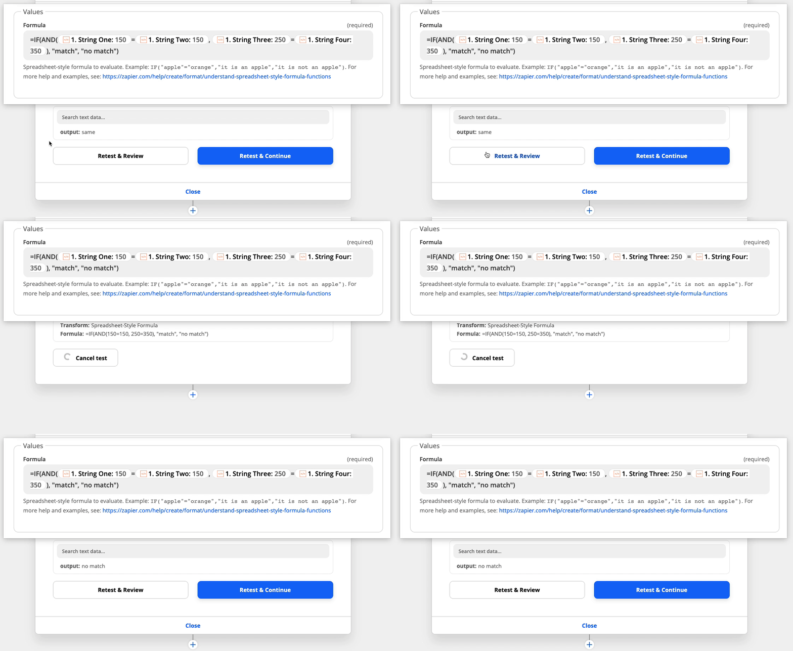
You can also compare two SETS of strings to see if they BOTH match. If they do, output value #1. Otherwise, output value #2.
=IF(AND("string1"="string2", "string3"="string4"), "match", "no match")
In a Zap:
IF / OR | String A Matches String 2 OR String 3 Matches String 4, Output Value 1, Otherwise Output Value 2
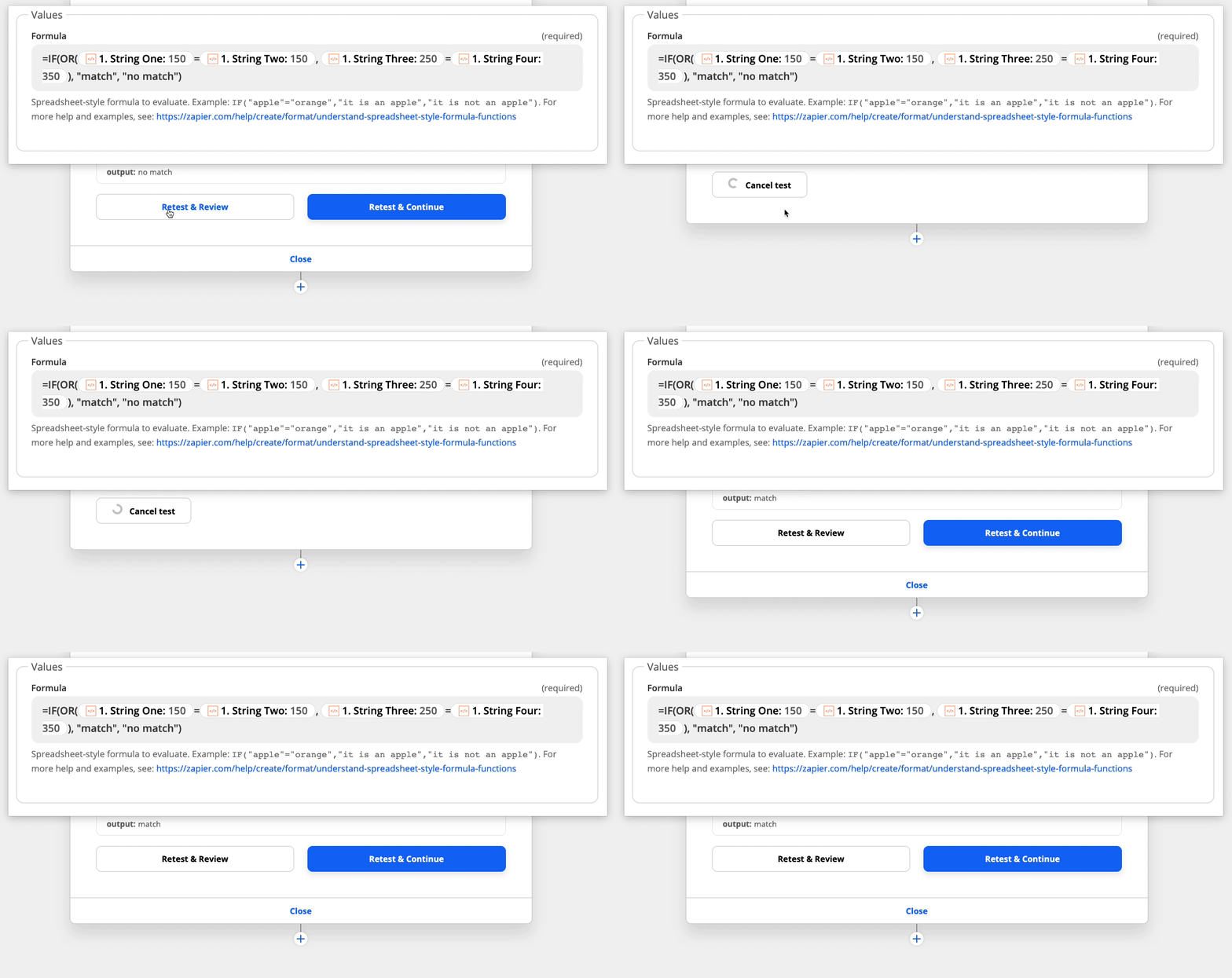
This is similar to the example above, except that matching BOTH of the sets of comparisons, you just need ONE of them to match. If so, output value #1. If no sets match, output value #2.
=IF(OR("string1"="string2", "string3"="string4"), "a match", "no matches")
In a Zap:
As I mentioned above, you can check for more than exact matches between values. You can see if something is NOT equal, is greater than (or equal to), is less than (or equal to).
Time to Tackle Something More Complex
Let’s jump into something a bit trickier and less obvious at first glance.
Outputting Letter Grades Based on Class Scores
Here we’re going to look at the grades in two different classes, and if both of them are greater than 90 we’ll output A. If not, we’ll then see if they’re above 85 and output a B. Then 80 for C and 75 for D.
And yes, I know these are not the actual percentages for those letter grades. I just made it up for demonstration purposes.

Here you can see it color-coded, to make it a bit more obvious which pieces belong together. So we would check in this order: yellow, green, pink, purple. Whichever one matches first is what we’ll output.

Outputting a Full City Name Based on Multiple Possible Versions
Let’s say you’re asking for a city name and you notice that for Atlanta, people are entering a few variations:
- Atlanta
- AT
- ATL
- Atl
- atl
- Atla
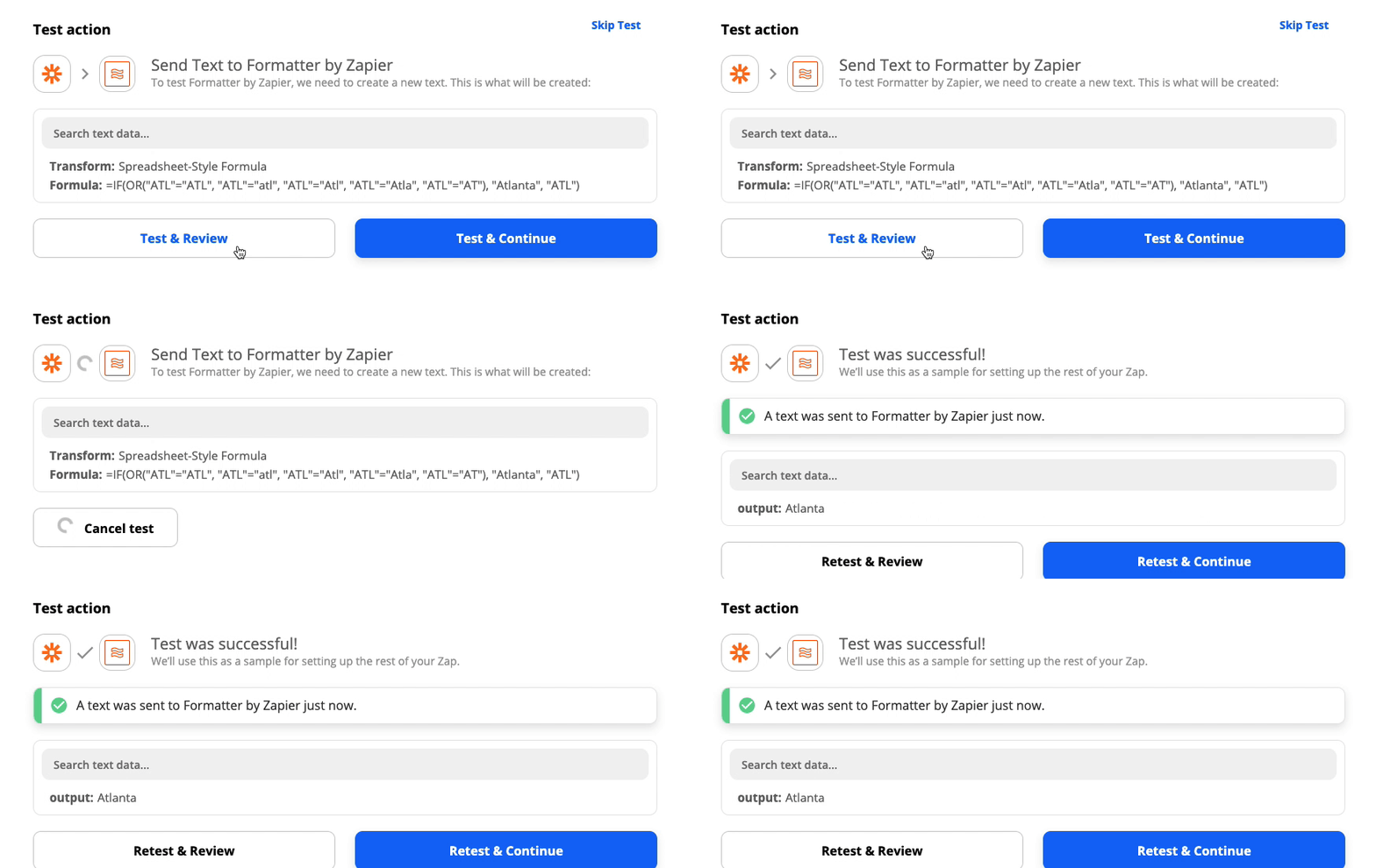
If any of those options are used, you’d like to output “Atlanta”. Otherwise, we’ll output the value that the person entered. Using what we learned earlier, let’s see if we c na figure this one out.
We saw this: =IF(OR("string1"="string2", "string3"="string4"), "a match", "no matches")
It should just be a matter of adding a few more conditions in there.

Alright, let’s test it out and see if it works:
Combining IF Function with Average
Similar to our first example, I’m going to look at grade. In this case, I want to take the average of 3 classes and depending what the result is, I want to output “Good”, “Satisfactory” or “Poor”.

TIP: Make sure you know the syntax of the particular function you’re using. When I first set up this Zap, I used =IF(AVERAGE(Algebra + Chemistry + Physics)… with the + symbols instead of the commas.
Other Resources
If you’re looking for more information, here are a few places you can look:
- Community articles
- Zapier’s help docs (here + here)
- This video from the first version of Zapier University
Wrapping Up
Hopefully this article has given you enough examples and explanations to help you use spreadsheet-style formulas a little more confidently :) We’d love to hear about how you’re using this feature in your Zaps!


