Hello! I have recorded a short 1min video explaining what I am trying to do.
https://www.loom.com/share/1cd34826fba64731a456bd14ba3df5d2
Deep THANK YOU to whoever can help me with this. Thank you so much :)
Derek

Hello! I have recorded a short 1min video explaining what I am trying to do.
https://www.loom.com/share/1cd34826fba64731a456bd14ba3df5d2
Deep THANK YOU to whoever can help me with this. Thank you so much :)
Derek
Best answer by PaulKortman
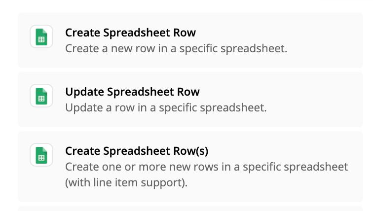
so I’d set up a google sheet to have 4 columns, Name, Qty, Order #, Formula1, and Formula2
I would have a step in zapier Google Sheets > Create new row(s) and put the line items name in the first column, the line items quantity in the second column and the order # in the third column. in the fourth column (Formula1) I would put the following formula
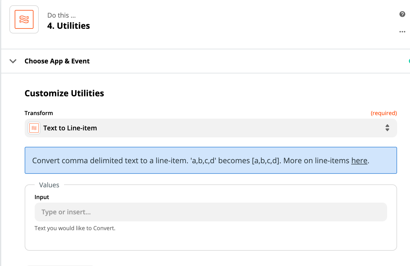
=if(find("salad","{{line item name}}")>0,{{line item qty}},if(find("bowl","{{line item name}}")>0,{{line item qty}},""))Note: I’ve never tried this with line items in a formula like this so that formula might not work, if not see the alternative formula option below.
Then I would add an additional step that find multiple rows where the Order # = the order number of this order (from shopify). You will then have the Quantities you need to add up in the Formula column.
Alternative Formula Idea:
Instead of writing the formula using Zapier, you could use the following which is Google sheet’s methodology and copy it down from row 2 to the 1000th row in the sheet - not ideal because it will eventually run out.
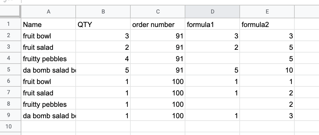
=if(iferror(find("salad",A2),false),B2,if(iferror(find("bowl",A2),false),B2,""))you could then add the following formula to the 5th column and copy this down
=if(c1=c2,e1+d2,d2)this formula2 basically reads, if the order number of this row (c2) equals the order number of the row above (c1) then add the formula1 of this row (d2) to the formula2 of the row above (e1). If this row’s order number does not equal the row’s order number above it then just put the results of this row (d2).
Then you can change the search step in Zapier Google Sheets to just look for one row and search from the bottom up, the last row in any given order number in the e column (formula2) will have the total number of salads and bowls.
Sometimes it’s easier to see it in action:
Enter your E-mail address. We'll send you an e-mail with instructions to reset your password.