Select a random row/value in a Google Sheet


Userlevel 7
Badge +12

Let's say you want to send yourself a random motivational message each day, and you have a collection of inspirational quotes in a Google Sheet. We want to build a Zap that will trigger each morning and choose one of the quotes to send to you on Slack. Here's how you can do that.

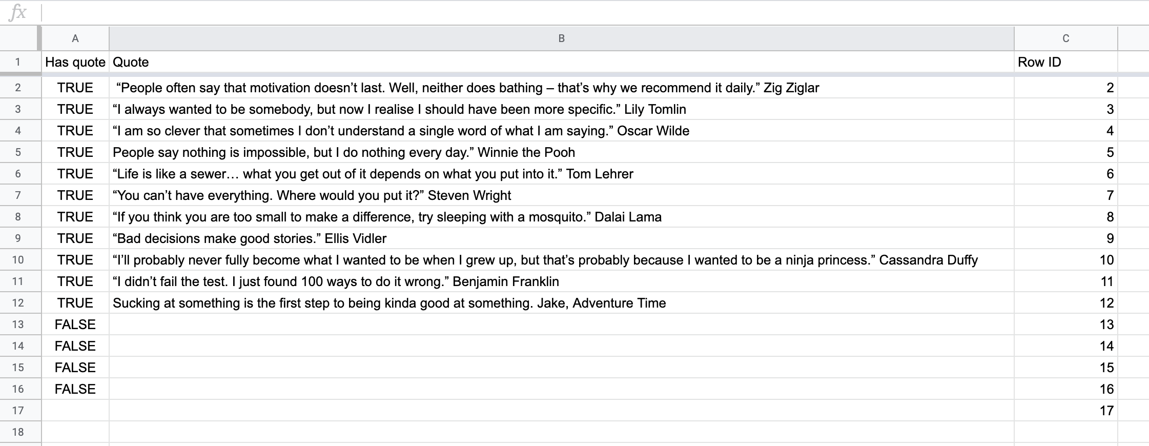
First, create your Google Sheet. For the first column, add the header 'Has quote' and have your quotes in the second column. In the first column, add this formula:

=if(ISBLANK(B2),FALSE,TRUE)

This will return the Value 'TRUE' if there's a quote in the quote column 'FALSE' if there isn't. You can copy this formula into every row - whether or not there's a quote in there now.

Add your quote in the second column, and then add a third column called 'Row ID'. This third column will tell the Zap which Google Sheets Row each quote is on, which we'll need.

image.png

Then create your Zap. In this case we're using Schedule as a trigger so that I can get an inspirational quote once a day.

The next step is a Google Sheets Lookup Spreadsheet Row action. Set up the step so that it is looking in the Has Quote column for the value 'FALSE'. That means that it will always find the first row in the sheet that doesn't have a quote in it.

Now we need a step that will generate a random row number. To do that, we'll use the Formatter by Zapier app choosing the 'Spreadsheet Style Formula' option in 'Numbers'. For the formula, we use:

image.png
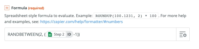
This tells the Zap to pick a random number between 2 and the Row ID number from the previous step, minus 1. We're starting at 2 because Row 1 is the header row.

Now let's pick that quote!

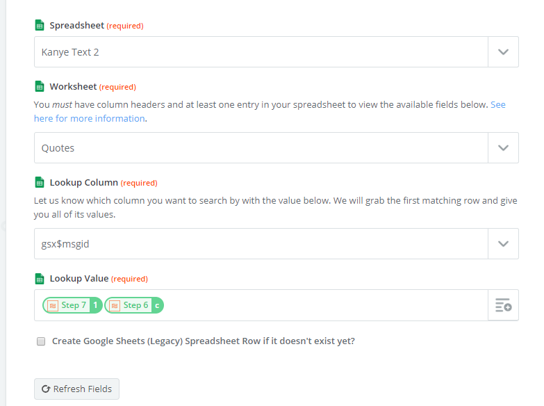
Add another Lookup Spreadsheet Row step. This time, set the Lookup Column to the Row ID column and the Lookup value to be the output of the Formatter step.

image.png
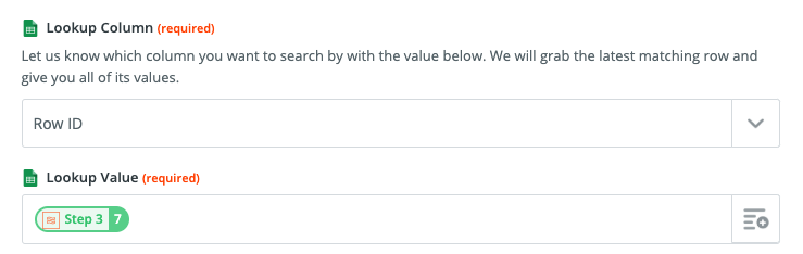
With this set up, each time the Zap runs, it will find the last row in the sheet and then choose a random row between the first and last row with a quote in it.

Finally we can add the Slack action to send the quote. Obviously, you can use any action you like here!


13 replies

Userlevel 2

Great walk through. We used a similar process when creating KanyeText.com - as it was all run through Zapier.

The main difference for us was that we wanted to select from one of three random quotes, per message. So picking from a random list, but still having some control over the results.

In other words:

Message one was either 1a, 1b, 1c

Message two was 2a, 2b, 2c

etc.

Our Steps were

  1. So we set up a new column in the google sheet with a list of 1a 1b 1c, all the way down to 100c.
  2. We used the utillities to pick from a list, selecting a random value. We had a, b, c (see image one)
  3. We have a payment sheet, that listed how many messages they had purchased and how many messages had been sent
  4. We incremented the number of messages that had been sent - 1 becomes 2, 2 became 3, 3 became 4 and so on
  5. We then did a lookup in google sheet for the column and put together the incriminated value and the A B C (see image 2)


image.pngimage.pngWe put a 54 minute video together that shows you how to build KanyeText but the guide is here https://medium.com/code-without-code/build-your-own-trumptext-in-less-than-an-hour-9bd9686a3dd7


Userlevel 7
Badge +12

What an interesting Zap! Thanks for sharing


Userlevel 2

Hey, @Danvers

Really liked the idea of this Zap so I tried to replicate it. I got stuck in the second Lookup Spreadsheet Row step where you set the Lookup Column to Row ID.

Do you have a third column in the spreadsheet called Row ID that duplicates row numbers? If so, how do you make Zapier find the actual quote in the random row instead of just the duplicated Row ID value?

From your tutorial it seems like I should be able to look up a cell value in a specific column by row ID. However in Zapier it looks like I can only do the opposite - namely, to look up a row ID by a cell value in a specific column, which is what you do in your first lookup step.


Userlevel 7
Badge +12

Hi @viesturs! How embarrassing, you're right I completely forgot to mention the extra column 😱

Yes, you do need one last column in the table that has the ID of each row in it. I'm so sorry that I forgot to add that initially, I'm going to edit the post now to make that super clear. Thanks for catching my omission and I hope it didn't cause you too much trouble!


Userlevel 2

@Danvers No worries, thanks for the clarification 🙂


Userlevel 4
Badge +2

Thank you for posting this. Every month we have a step count challenge and I've been wondering how to approach picking three winners at random using Zapier and Airtable or a G Sheet.


Userlevel 1

This was super helpful, thank you @Danvers!

I have a similar zap for question of the day that posts to Slack. We have now found that it is repeating questions often, even though it has not run through the entire list. Is there a way to tell it to take the question/quote out of rotation after it has been used? I am stump on this one. Thanks, 


John

Userlevel 7
Badge +7

Hi @John_Hero I think I can help you out a bit.

Try to think about such an issue a different way, in this case not about removing it, but adding it to another “list”. What you could do is the following:

  • Add another column in the sheets called something like “used”
  • Within the last “Lookup Spreadsheet Row” step add a supporting search term looking at this new “used” column
  • Search for the value FALSE
  • After the last step, add another Google Sheets step to “Update spreadsheet row”
  • On this step, use the row ID from the last step you used, and update the column “Used” to TRUE
  • Now when this whole zap workflow runs again, it should only find the quotes that have not been used yet

Let me know if this makes sense or if you need some more assistance. Hope this works for you!

~Bjorn

Thanks @ForYourIT,


That seems to have worked. I will need to watch it for a bit and double check, but I think we are on the right track.

Userlevel 7
Badge +7

Hi @John_Hero ,

Did that work for you or do you need any additional assistance? Feel free to hit me with some questions ;D


~ Bjorn

Hey there,

The original zap from this posted worked great. Similar to JohnHero discussed after, I don’t want to reuse the same rows if they have already been sent in slack. 

When I attempted to add the steps for this, the Zap broke. One thing that wasn’t mentioned in your steps was to add False to every cell in the “Used” row. Maybe I did something wrong with this. Next, the Random Number selector step takes place before the 2nd lookup row. The 2nd lookup row step is what determines if the cell has been used or not. The random number chose a row that already had the “used” column marked as “true” and this broke the 2nd lookup row.


Im not sure if I missed something in your instructions or not.


Thank you,


How do I create a Zap that every day looks up the next row in Google sheets?

I have a work-around that is a bit too complicated and I’m hoping for a simple and effective way with less than 3 steps.

To give you an example of a use case, I have a Google spreadsheet with motivational quotes on each row, and every day I want to send the next quote to Gmail. I don’t want to send the very latest quote at the bottom of the list, or a random quote from the list, only the next quote in the list.

Reply