Best answer

Using row number as ID but must be 3 digits starting at 001

  • 7 July 2020
  • 5 replies
  • 520 views

Userlevel 1

I have a trigger, when a new spreadsheet row is added. I take the row number (start at 2) because of the header. So the first value should be 2.

A format step will MINUS 1 from the Row number - giving me 1. This is the fist row after the column header.


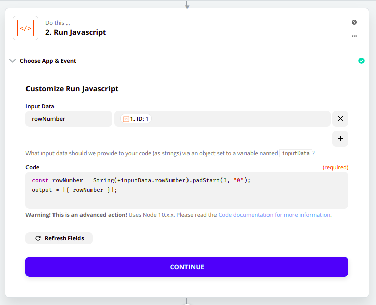
But I need to format the number to 3 digits, like 001.

When it hits 10, it the value should be 010, then 100 and so on.


Any ideas? Thank you!

icon

Best answer by ikbelkirasan 7 July 2020, 22:42

View original

This post has been closed for comments. Please create a new post if you need help or have a question about this topic.

5 replies

Userlevel 7
Badge +12

@Merci - This can be done easily with a Code step. Here is the code:

const rowNumber = String(+inputData.rowNumber).padStart(3, "0");
output = [{ rowNumber }];


Userlevel 1

@Merci - This can be done easily with a Code step. Here is the code:

 const rowNumber = String(+inputData.rowNumber).padStart(3, "0");
output = [{ rowNumber }];


Thanks! However, I need the 1st row after the column header to be ROW 001. Can you code MINUS 1 or should I add a format step?

Userlevel 7
Badge +12

@Merci - Sure, you can do it in the same code:

const rowNumber = String(+inputData.rowNumber - 1).padStart(3, "0");
output = [{ rowNumber }];


Userlevel 1

Thanks for the solution again. I looked at adding data to Google Sheets and formatting the Row number into 3 digits, but your solution is much more streamline for Zapier. If you’re interested, you can find it here: 

https://docs.google.com/spreadsheets/d/1oAtDLo2Bk-3SaUAYX9GrscC6DN_h8lO8pqLUWPTAoJw/edit?usp=sharing

A2 =ARRAYFORMULA(IF(B2:B="",,TEXT(ROW(data!A1:A), "000")))
B2 =ARRAYFORMULA(data!A2:B)


Userlevel 7
Badge +12

@Merci - Great, thanks for sharing!